You May Be Interested In… Ticketmaster Trends Post-Pandemic

The last concert I attended before the world pressed pause on large gatherings was Galantis’s Church of Galantis at San Francisco’s Bill Graham Civic Auditorium. One moment, I was in a sea of excitement; the next, I was sheltering in place. When concerts finally returned, masks had become fashionable accessories with special designs and bedazzles — though their use seems to have faded over time. Measuring changes like that is tough with data.

But one thing I can measure is interest in concert tickets.

The pandemic changed a lot — how we work, shop, and even Target’s store hours. I started wondering: did it also change people’s interest in attending concerts? As a proxy for ticket-buying interest, I looked at Google search data for the term “ticketmaster” in California, my home state.

Concerts Canceled

To set the scene: on March 11, 2020, California Governor Gavin Newsom issued a public health directive postponing events with 250 or more people until further notice. Some live music still found a way, like at drive-in concerts which were so fun! These restrictions were officially lifted on June 15, 2021.

To begin our analysis, I pulled monthly search interest data on the term “Ticketmaster” from Google Trends:

# Read in data
ticketmaster_data <- read_csv('multiTimeline.csv', skip=1) %>%
  mutate(Date=ymd(paste0(Month, '-15'))) %>%
  rename(`Search Count`=`ticketmaster: (California)`) %>%
  select(Date, `Search Count`)

Let’s take a peek at the first few rows:

# Preview
head(ticketmaster_data)

## # A tibble: 6 × 2
##   Date       `Search Count`
##   <date>              <dbl>
## 1 2015-05-15             65
## 2 2015-06-15             70
## 3 2015-07-15             70
## 4 2015-08-15             71
## 5 2015-09-15             71
## 6 2015-10-15             64

Breaking It Down: Pre-, During, and Post-Pandemic

To make sense of how interest in concert tickets changed, I divided the timeline into three periods:

1. Pre-pandemic (before March 11, 2020)

2. Pandemic (March 11, 2020 to June 15, 2021)

3. Post-pandemic (after June 15, 2021)

These labels aren’t perfect — life didn’t flip back to “normal” overnight — but they help anchor the analysis. We’ll make do.

Let’s take a look at the search summary statistics during each period.

# Create the `Period` variable
ticketmaster_data <- ticketmaster_data %>%
  mutate(Period=case_when(
    Date < '2020-03-11' ~ 'Pre-pandemic',
    Date > '2021-06-15' ~ 'Post-pandemic',
    TRUE ~ 'Pandemic'
  )) %>%
  mutate(Period=factor(Period, levels=c('Pre-pandemic', 'Pandemic', 'Post-pandemic')))

# Show summary statistics
ticketmaster_data %>%
  group_by(Period) %>%
  summarise(
    across(`Search Count`, list(
      mean = ~round(mean(.x), 2),
      sd = ~round(sd(.x), 2),
      min = ~round(min(.x), 2),
      q25 = ~round(quantile(.x, 0.25), 2),
      q50 = ~round(median(.x), 2),
      q75 = ~round(quantile(.x, 0.75), 2),
      max = ~round(max(.x), 2)
    ))
  )

## # A tibble: 3 × 8
##   Period        `Search Count_mean` `Search Count_sd` `Search Count_min`
##   <fct>                       <dbl>             <dbl>              <dbl>
## 1 Pre-pandemic                 57.6              10.2                 42
## 2 Pandemic                     12.7              13.9                  3
## 3 Post-pandemic                59.2              12.1                 31
## # ℹ 4 more variables: `Search Count_q25` <dbl>, `Search Count_q50` <dbl>,
## #   `Search Count_q75` <dbl>, `Search Count_max` <dbl>

Visualizing the periods paints the story even more vividly:

# Plot
ggplot(aes(x=Date, y=`Search Count`), data=ticketmaster_data) +
  geom_line(col='black', alpha=0.7) +
  geom_point(aes(col=Period)) +
  ggtitle('Searches of "ticketmaster" Before and After COVID-19 Directives') +
  theme_bw()

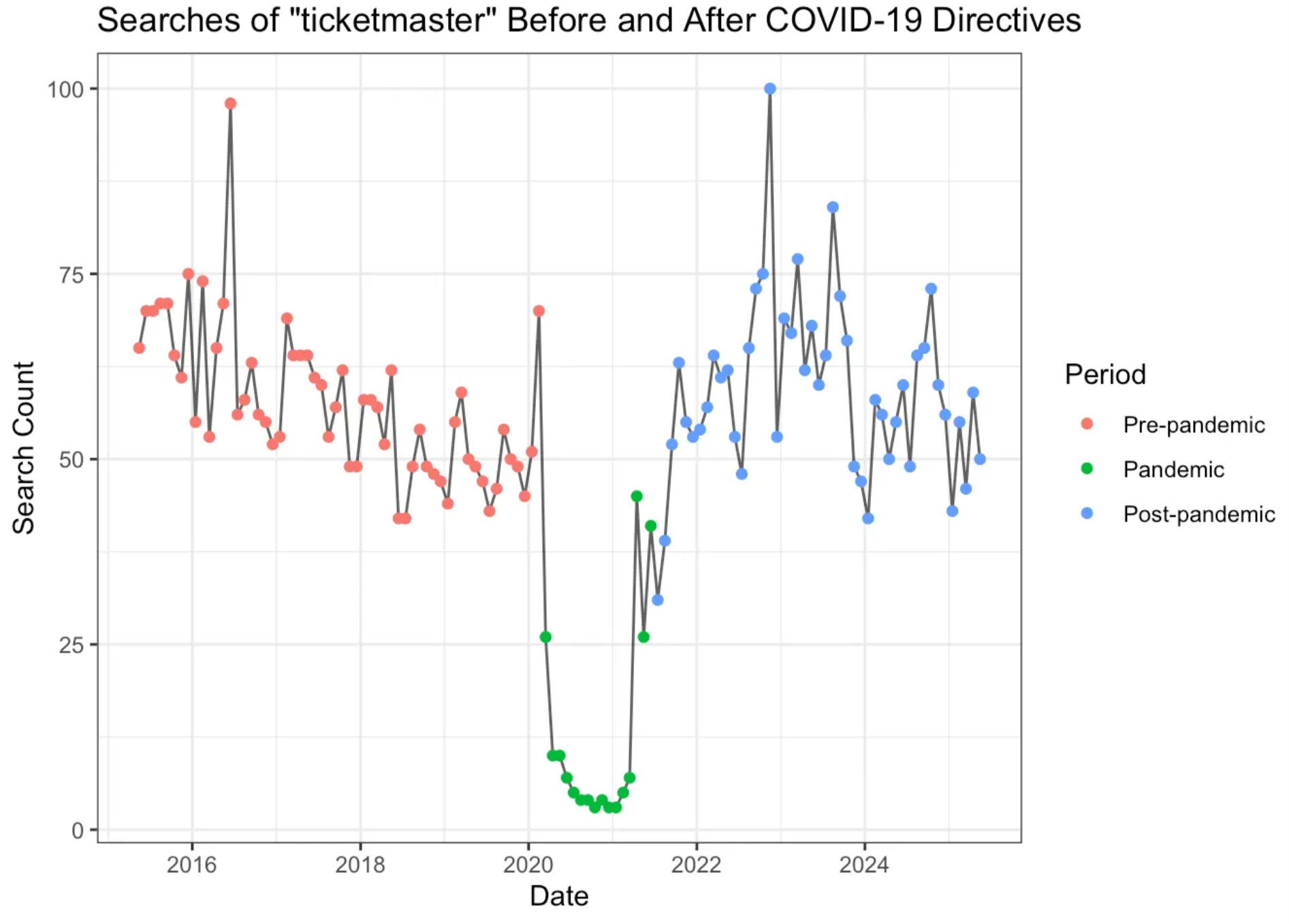
Over time, the term “ticketmaster” searches on Google changed. The pre-pandemic, pandemic, and post-pandemic eras had characteristic trends which we will uncover in this analysis.